Tutorials

Single Cell Transcriptomics with Seurat

Júlia Perera-Bel (MARData-BU, Hospital del Mar Research Institute)

Requirements
Introduction to Single Cell Transcriptomics
- Preprocessing with Cell Ranger
- Seurat
Loading data and initial QC
- Visualizing QC
- Cell filtering
Normalization and Scaling
Dimentionality reduction
Integration
Cell clustering
Annotation
- Using reference markers
- Using a reference
Differential expression
- FindAllMarkers and FindMarkers
- Pseudobulk Differential Expression

Requirements

This tutorial will be done with R with Seurat 5 R package.

Seurat depends on Matrix package. It is recommended to have Matrix version higher than 1.5), which requires R ≥ 4.4.

Other packages will be used for visaulization, annotation and functional enrichment

RStudio (or Visual Studio) is also recommended for interactive development.

install.packages("Matrix")
install.packages("Seurat")
Install.packages("ggplot2") 
remotes::install_github("satijalab/seurat-data") 
SeuratData::InstallData("ifnb") 
BiocManager::install("clusterProfiler") 

library(Matrix)
library(Seurat)
library(ggplot2)

Introduction to Single Cell Transcriptomics

scRNA-seq measures the abundance of mRNA molecules per cell. Extracted biological tissue samples constitute the input for single-cell experiments. Tissues are digested during single-cell dissociation, followed by single-cell isolation to profile the mRNA per cell separately. Plate-based protocols isolate cells into wells on a plate, whereas droplet-based methods capture cells in microfluidic droplets.

The obtained mRNA sequence reads are mapped to genes and cells of origin in raw data processing pipelines that use either cellular barcodes or unique molecular identifiers (UMIs) and a reference genome to produce a count matrix of cells by genes (Fig. 2a). You can find a detailed overview of single cell sequencing in the Single-Cell Best Practices online book. Here we will give a brief description of the preprocessing and consider count matrices as the starting point for our analysis workflow of scRNA-seq data.

Preprocessing with Cell Ranger

Cell Ranger is the commercial software from 10x Genomics. It comrpises a set of analysis pipelines that perform sample demultiplexing, barcode processing, single cell 3’ and 5’ gene counting, V(D)J transcript sequence assembly and annotation, and Feature Barcode analysis from single cell data.

For this tutorial we will be using data generated with the cellranger count pipeline. The input you need to run cellranger count are the sequence reads and a reference. The reference has a specific format. You can download precomputed human and mouse references from the 10X website.

cellranger count --id=$name --fastqs=$FASTQDIR --transcriptome=$REFDIR --sample=$base_name --create-bam=true --include-introns=true

The cellranger count pipeline outputs are in the pipestance directory in the outs folder. List the contents of this directory with ls -1.

├── analysis
├── cloupe.cloupe
├── filtered_feature_bc_matrix
├── filtered_feature_bc_matrix.h5
├── metrics_summary.csv
├── molecule_info.h5
├── possorted_genome_bam.bam
├── possorted_genome_bam.bam.bai
├── raw_feature_bc_matrix
├── raw_feature_bc_matrix.h5
└── web_summary.html

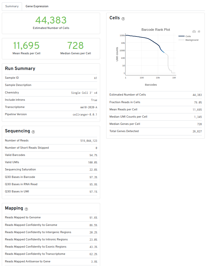
The web_summary.html contains a summary of the QC and results of the experiment. You can also load the cloupe.cloupe file into the Loupe Browser and start an analysis. The outs/ directory contains the outputs that can be used as input for software tools developed outside of 10x Genomics, such as the Seurat R package.

QC

It is common in droplet-based protocols that certain barcodes are associated with ambient RNA instead of the RNA of a captured cell. This happens when droplets fail to capture a cell. Many approaches exist to assess whether a barcode likely corresponds to an empty droplet or not.

One simple method implemented in CellRanger is to examine the cumulative frequency plot of the barcodes, in which barcodes are sorted in descending order of the number of distinct UMIs with which they are associated. This plot often contains a “knee” that can be identified as a likely point of discrimination between properly captured cells and empty droplet. While this “knee” method is intuitive and can often estimate a reasonable threshold, not all cumulative histograms display an obvious knee. Finally, the total UMI count associated with a barcode may not, alone, be the best signal to determine if the barcode was associated with an empty or damaged cell.

web_summary

There are several tools specifically designed to detect empty or damaged droplets, or cells generally deemed to be of “low quality”. We recommend importing all cells in R and filter empty droplets during the first quality check, in which several filters and heuristics are applied to obtain robust cells and genes. We also recommend to use SoupX for quantifying the extent of the contamination and estimating “background-corrected” cell expression profiles.

Seurat

The next step after the generation of the count matrices with cellranger count, is the data analysis. The R package Seurat is currently the most popular software to do this. To start working with Seurat you can load the data in two ways:

Using the barcodes/features/matrix files:

filtered_feature_bc_matrix
  ├── barcodes.tsv.gz
  ├── features.tsv.gz
  └── matrix.mtx.gz
  
raw_feature_bc_matrix
  ├── barcodes.tsv.gz
  ├── features.tsv.gz
  └── matrix.mtx.gz

Using h5 files:

raw_feature_bc_matrix.h5
filtered_feature_bc_matrix.h5

# folder with the three barcodes, features and matrix files
sc <- Read10X(file.path(dir,"raw_feature_bc_matrix")) 
# h5 file
sc <- Read10X_h5(file.path(dir,"raw_feature_bc_matrix.h5"))

Loading data and initial QC

In this tutorial we will be using scRNASeq data from lamina propia from the article by Martin et al. The data is available under the accession GEO GSE134809.

To speed up the tutorial, we will directly download the merged_seurat.Rds object and save it in a folder called GSE134809. Also, in case some steps of the tutorial don’t work, we have saved all objects generated in the tutorial here: R objects

Load the merged_seurat.Rds object:

data_dir="GSE134809"
merged_seurat <- readRDS(file.path(data_dir, "merged_data.Rds"))

Alternatively, if you want to learn to load the data from the raw cellRanger files, you can download the raw data through this link GSE134809 and then load the data with the following code:

# Download dataset
data_dir="GSE134809"
samples=list.files(data_dir,pattern = "GSM")
metadata=read.delim2(file.path(data_dir,"Metadata.csv"))
#Creato list to store the data
seurat_list=list()

for (name in samples){
  cat(paste("\n Readding sample", name, "\n", sep = " "))
  temp_dir <- file.path(data_dir, name)
  # Now Read10X
  counts <- Read10X(data.dir = temp_dir)
  
  # Create Seurat object
  seurat_obj <- CreateSeuratObject(counts = counts, project = name, min.cells = 3, min.features = 200)
  # Add sample info
  seurat_obj$name <- name
  seurat_obj$tissue <- metadata$tissue[metadata$GEO_ID==name]
  seurat_obj$status <- metadata$status[metadata$GEO_ID==name]
  seurat_obj$Sample_ID <- metadata$Sample_ID[metadata$GEO_ID==name]
  seurat_obj$Patient <- metadata$Patient[metadata$GEO_ID==name]
  seurat_obj$Chemistry <- metadata$Chemistry[metadata$GEO_ID==name]

  # calculate % of mithocondrial RNA
  seurat_obj$percent.mt <- PercentageFeatureSet(seurat_obj, pattern = "^MT-") 
  # calculate % of ribosomal RNA
  seurat_obj$percent.rp <- PercentageFeatureSet(seurat_obj, pattern = "^RPL|^RPS") 
  
  # Store it
  seurat_list[[name]] <- seurat_obj
  
}

# Merge all Seurat objects into one
merged_seurat <- merge(x = seurat_list[[1]], y = seurat_list[2:length(seurat_list)],add.cell.ids = names(seurat_list))


saveRDS(merged_seurat, file.path(data_dir, "merged_data.Rds"))

# Free space and memory
rm(seurat_list,seurat_obj,counts)

Let’s explore the Seurat object.

merged_seurat

## An object of class Seurat 
## 21939 features across 70616 samples within 1 assay 
## Active assay: RNA (21939 features, 0 variable features)
##  12 layers present: counts.GSM3972009, counts.GSM3972010, counts.GSM3972013, counts.GSM3972014, counts.GSM3972017, counts.GSM3972018, counts.GSM3972021, counts.GSM3972022, counts.GSM3972025, counts.GSM3972026, counts.GSM3972027, counts.GSM3972028

# Check cell metadata
head(merged_seurat@meta.data) #dataframe

##                             orig.ident nCount_RNA nFeature_RNA       name
## GSM3972009_AAACATACACACCA-1 GSM3972009       1233          500 GSM3972009
## GSM3972009_AAACATTGGTGTCA-1 GSM3972009       4142         1275 GSM3972009
## GSM3972009_AAACGCACTTAGGC-1 GSM3972009       5806         1726 GSM3972009
## GSM3972009_AAACGCTGAGAATG-1 GSM3972009        695          274 GSM3972009
## GSM3972009_AAACGCTGCTACCC-1 GSM3972009       1329          626 GSM3972009
## GSM3972009_AAACGCTGCTCATT-1 GSM3972009        896          358 GSM3972009
##                             tissue   status Sample_ID Patient Chemistry
## GSM3972009_AAACATACACACCA-1  ILEUM Involved        69       5        V1
## GSM3972009_AAACATTGGTGTCA-1  ILEUM Involved        69       5        V1
## GSM3972009_AAACGCACTTAGGC-1  ILEUM Involved        69       5        V1
## GSM3972009_AAACGCTGAGAATG-1  ILEUM Involved        69       5        V1
## GSM3972009_AAACGCTGCTACCC-1  ILEUM Involved        69       5        V1
## GSM3972009_AAACGCTGCTCATT-1  ILEUM Involved        69       5        V1
##                             percent.mt percent.rp
## GSM3972009_AAACATACACACCA-1  1.2165450   33.81995
## GSM3972009_AAACATTGGTGTCA-1  1.2554322   18.80734
## GSM3972009_AAACGCACTTAGGC-1  0.6717189   17.58526
## GSM3972009_AAACGCTGAGAATG-1  2.8776978   41.15108
## GSM3972009_AAACGCTGCTACCC-1  1.0534236   15.65087
## GSM3972009_AAACGCTGCTCATT-1  1.4508929   39.62054

# Set primary cell identity to Sample_ID
Idents(merged_seurat) <- merged_seurat$Sample_ID

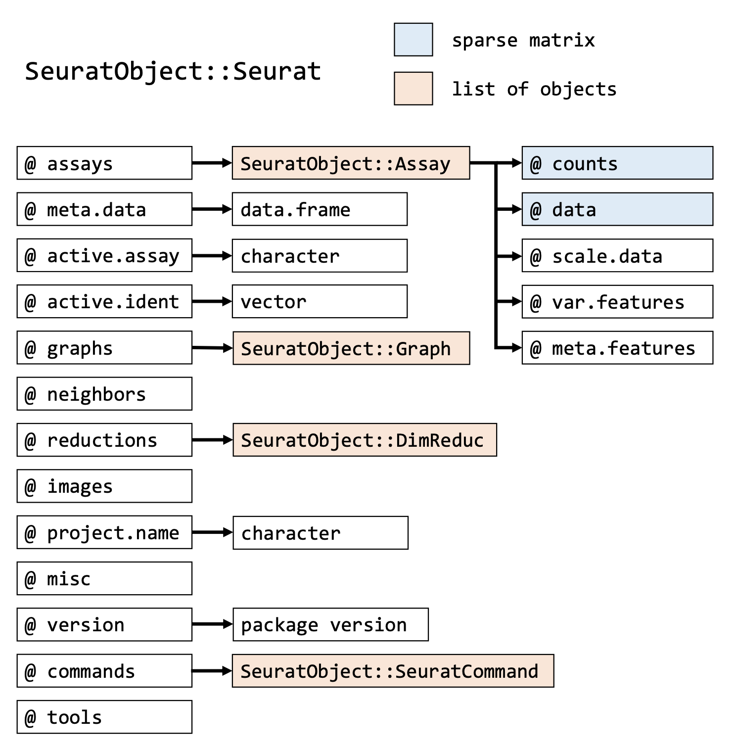
Each Seurat object contains exactly the same slots that are specified in the image below. You can get the information inside a slot with @, in the same way as you would use the $ for lists. In addition to the original count table, the Seurat object can therefore store a lot of information that is generated during your analysis, like results of a normalization (@assays$RNA@data) a PCA or UMAP (@reductions) and the clustering (@graphs). It also tracks all the commands that have been used to generate the object in its current state (@commands). Therefore, while going through the analysis steps, the same object gets more and more of its slots filled.

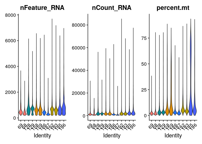
Visualizing QC

While generating the Seurat object, there were already some quality measures calculated for each cell, namely the total UMI counts per cell (nCount_RNA) and the total number of detected features per cell (nFeature_RNA).

nFeature: The number of unique genes detected in each cell. Low-quality cells or empty droplets will often have very few genes. Cell doublets or multiplets may exhibit an aberrantly high gene count.
nCount: Similarly, the total number of molecules detected within a cell (correlates strongly with unique genes)

We can also calculate other useful metrics and use for filtering cells include:

Mitochondrial genes: If a cell membrane is damaged, it looses free RNA quicker compared to mitochondrial RNA, because the latter is part of the mitochondrion. A high relative amount of mitochondrial counts can therefore point to damaged cells.

All of them can be plot in a violin plot and evaluate their distribution per sample:

VlnPlot(merged_seurat, features=c("nFeature_RNA","nCount_RNA","percent.mt"), pt.size = 0,split.by = "Patient")

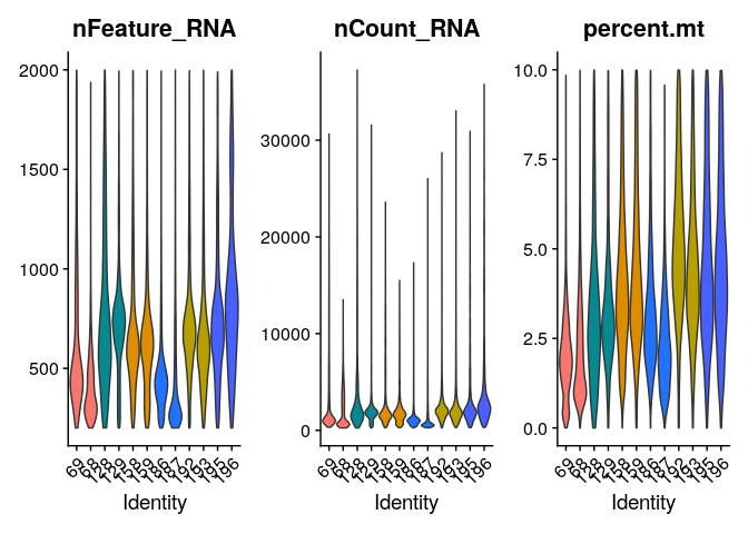
Cell filtering

Based on the QC process we went through we can come to the following conclusions:

Two samples present high mitochondrial gene counts.
There are some cells with a very low and very high number of features. These might point to non-informative cells and doublets respectively.

In the M\&M of the publication], the authors do not describe the thresholds used to filter cells. Observing the distribution of the plots, we suggest a threshold of < 10% mitochondrial counts and > 200 features per cell. To filter against possible doublets, here, we also filter out cells with > 2000 detected features/cell. Filtering Seurat objects can be done with the subset method for class SeuratObject:

merged_seurat_filt <- subset(merged_seurat, subset = nFeature_RNA > 200 & 
                               nFeature_RNA < 2000 &
                               percent.mt < 10)

We can compare the number of filtered cells:

cbind(table(merged_seurat$orig.ident),table(merged_seurat_filt$orig.ident))

##             [,1]  [,2]
## GSM3972009  3739  3553
## GSM3972010 11488 11199
## GSM3972013  3273  2756
## GSM3972014  2743  2155
## GSM3972017  5534  3339
## GSM3972018  6237  3009
## GSM3972021  6423  6007
## GSM3972022  3010  2952
## GSM3972025  9073  6357
## GSM3972026 10537  8970
## GSM3972027  4666  1844
## GSM3972028  3893  2088

To evaluate this did the trick we can visualize those parameters again in a violin plot:

VlnPlot(merged_seurat_filt, features = c("nFeature_RNA","nCount_RNA","percent.mt"),pt.size = 0,split.by = "Patient")

#we remove non filtered seurat object
rm(merged_seurat)

Normalization and Scaling

The preprocessing step of normalization aims to adjust the raw counts in the dataset for variable sampling effects by scaling the observable variance to a specified range. Several normalization techniques are used in practice varying in complexity. By default, Seurat employs a global-scaling normalization method “LogNormalize” that normalizes the feature expression measurements for each cell by the total expression, multiplies this by a scale factor (10,000 by default), and log-transforms the result. Normalized values are stored in the “RNA” assay (as item of the @assay slot) of the seu object.

We next identify the highly variable features (i.e, they are highly expressed in some cells, and lowly expressed in others). Focusing on these genes in downstream analysis helps to highlight biological signal in single-cell datasets and reduces computational cost. Seurat’s procedure directly models the mean-variance relationship inherent in single-cell data, and is implemented in the FindVariableFeatures() function. By default, the function returns 2,000 features per dataset. These will be used in downstream analysis, like PCA.

Next, we apply scaling, a linear transformation that is a standard pre-processing step prior to dimensional reduction techniques like PCA. The ScaleData() function shifts the expression of each gene, so that the mean expression across cells is 0 and the variance across cells is 1. This step gives equal weight in downstream analyses, so that highly-expressed genes do not dominate. The results of this are stored in <seu$RNA@scale.data> By default, only variable features are scaled.

We can also use the ScaleData() function to remove unwanted sources of variation from a single-cell dataset. For example, we could regress out heterogeneity associated with (for example) cell cycle stage, or mitochondrial contamination. Here you can find a tutorial to regress out cell cycle scores.

For advanced users, there is an alternative normalization workflow, SCTransform(), described here, that does not rely on the assumtion that each cell originally contains the same number of RNA molecules. The use of SCTransform replaces the need to run NormalizeData, FindVariableFeatures, or ScaleData. Also, as with ScaleData(), the function SCTransform() also includes a vars.to.regress parameter.

merged_seurat_filt <- NormalizeData(merged_seurat_filt)
merged_seurat_filt <- FindVariableFeatures(merged_seurat_filt)
merged_seurat_filt <- ScaleData(merged_seurat_filt) # needs some RAM

Dimentionality reduction

Perform linear dimensional reduction

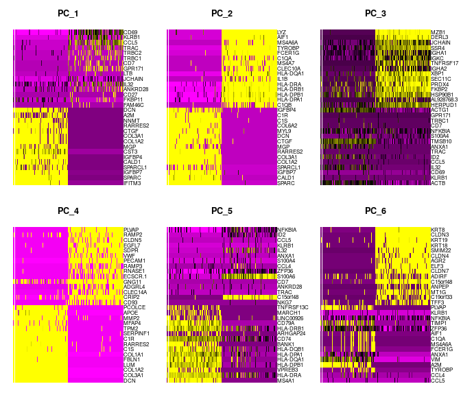
Next we perform PCA on the scaled data. By default, only the previously determined variable features are used as input, but can be defined using features argument if you wish to choose a different subset (if you do want to use a custom subset of features, make sure you pass these to ScaleData first).

For the first principal components, Seurat outputs a list of genes with the most positive and negative loadings, representing modules of genes that exhibit either correlation (or anti-correlation) across single-cells in the dataset. These can be visualized by heatmaps:

merged_seurat_filt <- RunPCA(merged_seurat_filt)

DimHeatmap(merged_seurat_filt, dims = 1:6, cells = 500, balanced = TRUE)

Determine the ‘dimensionality’ of the dataset

The elbowplot can help you in determining how many PCs to use for downstream analysis such as UMAP, by finding the flattening point (elbow) in which the majority of true signal is captured. However, a useful automatic way to determine the optimal number of principal components (PCs) to retain is depicted below:

ElbowPlot(merged_seurat_filt)

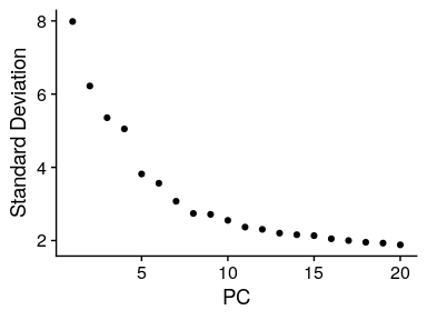
# Calculate optimal number of PC to use for the clustering
pct <- merged_seurat_filt[["pca"]]@stdev / sum(merged_seurat_filt[["pca"]]@stdev) * 100
cumu <- cumsum(pct)
# Find the first PC where cumulative variance > 90% and the PC itself explains < 5% of the variance
co1 <- which(cumu > 90 & pct < 5)[1]
# Find the first PC where the drop in variance explained between consecutive PCs is > 0.1%
co2 <- sort(which((pct[1:length(pct) - 1] - pct[2:length(pct)]) > 0.1), decreasing = T)[1] + 1
# Take the more conservative estimate (lower value) between the two
co3 <- min(co1, co2) # 11

Run non-linear dimensional reduction (UMAP/tSNE)

Non-linear dimensional reduction methods capture complex, non-linear relationships between cells that linear methods (like PCA) might miss. Two methods are implemented in Seurat:

UMAP (Uniform Manifold Approximation and Projection): The goal is to learn the underlying manifold of the data in order to place similar cells together in low-dimensional space. UMAP preserves spatial structure.
t-SNE (T-distributed stochastic neighbour embedding): focuses on preserving local similarities while potentially distorting global distances.

merged_seurat_filt <- RunUMAP(merged_seurat_filt, reduction="pca", dims=1:co3, reduction.name = "umap.unintegrated")
merged_seurat_filt <- RunTSNE(merged_seurat_filt, reduction="pca", dims=1:co3, reduction.name = "tsne.unintegrated")

saveRDS(merged_seurat_filt, file.path(data_dir, "merged_data_filt.Rds"))

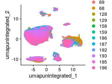
Having a look at the UMAP and t-SNE, can observe that although cells of different samples are shared amongst “clusters”, you can still see “sample-specific” clusters:

# We can compare between PCA, UMAP and tSNE methods
DimPlot(merged_seurat_filt, reduction = "pca")

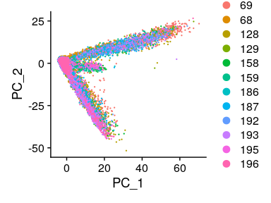
DimPlot(merged_seurat_filt, reduction = "umap.unintegrated")

DimPlot(merged_seurat_filt, reduction = "tsne.unintegrated")

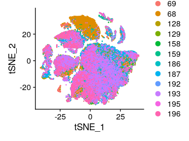
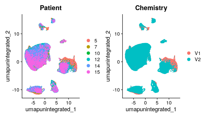
Having a look at the UMAP and t-SNE, can observe that although cells of different samples are shared amongst “clusters”, you can still see “sample-specific” clusters. Separating by technical variables shows that Chemistry is introducing a batch effect.

#We can explore the different metadata and identify the need to integrate
DimPlot(merged_seurat_filt, reduction = "umap.unintegrated",group.by = c("Patient","Chemistry"))

Integration

Seurat v5 enables streamlined integrative analysis using the IntegrateLayers function. The method currently supports five integration methods. Each of these methods performs integration in low-dimensional space, and returns a dimensional reduction (i.e. integrated.rpca) that aims to co-embed shared cell types across batches:

Anchor-based CCA integration (method=CCAIntegration)
Anchor-based RPCA integration (method=RPCAIntegration)
Harmony (method=HarmonyIntegration)
FastMNN (method= FastMNNIntegration)
scVI (method=scVIIntegration)

Note that anchor-based RPCA integration represents a faster and more conservative (less correction) method for integration.

# Integrate
dwIntegrated <- IntegrateLayers(
  object = merged_seurat_filt, method = RPCAIntegration,
  orig.reduction = "pca", new.reduction = "integrated.rpca",
  verbose = TRUE
)

#Run dimensionality reduction on integrated.rpca
dwIntegrated <- RunUMAP(dwIntegrated, reduction="integrated.rpca", dims=1:co3, 
                        reduction.name = "umap.integrated")

# save integrated object
saveRDS(dwIntegrated, file.path(data_dir, "integrated_data.Rds"))

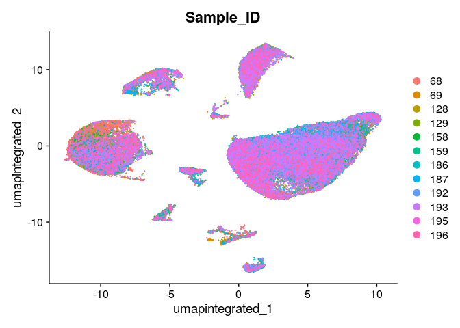
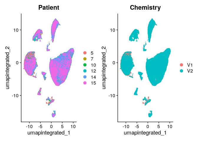
Evaluate with UMAP if the integration removed the technical effects:

DimPlot(dwIntegrated, reduction = "umap.integrated",group.by = "Sample_ID")

DimPlot(dwIntegrated, reduction = "umap.integrated",group.by = c("Patient","Chemistry"))

# Remove uninegrated object
rm(merged_seurat_filt)

Cell clustering

The method implemented in Seurat first constructs a SNN graph based on the euclidean distance in PCA space, and refine the edge weights between any two cells based on the shared overlap in their local neighborhoods (Jaccard similarity). This step is performed using the FindNeighbors() function, and takes as input the previously defined dimensionality of the dataset.

To cluster the cells, Seurat next implements modularity optimization techniques such as the Louvain algorithm (default) or SLM [SLM, Blondel et al., Journal of Statistical Mechanics], to iteratively group cells together, with the goal of optimizing the standard modularity function. The FindClusters() function implements this procedure, and contains a resolution parameter that sets the ‘granularity’ of the downstream clustering, with increased values leading to a greater number of clusters.

dwIntegrated <- FindNeighbors(dwIntegrated, reduction="integrated.rpca", dims=1:co3) # reduce k.param and dims to make it quicker
dwIntegrated <- FindClusters(dwIntegrated, resolution=0.5) # try different resolutions

# Rejoin (collapse) the layers, needed for downstream analysis
dwIntegrated <- JoinLayers(dwIntegrated, assay = "RNA")

saveRDS(dwIntegrated, file.path(data_dir, "integrated_data.Rds"))

We look at the resulting clusters in the UMAP:

Idents(dwIntegrated) <- dwIntegrated$seurat_clusters
DimPlot(dwIntegrated, reduction = "umap.integrated",label=T)

Annotation

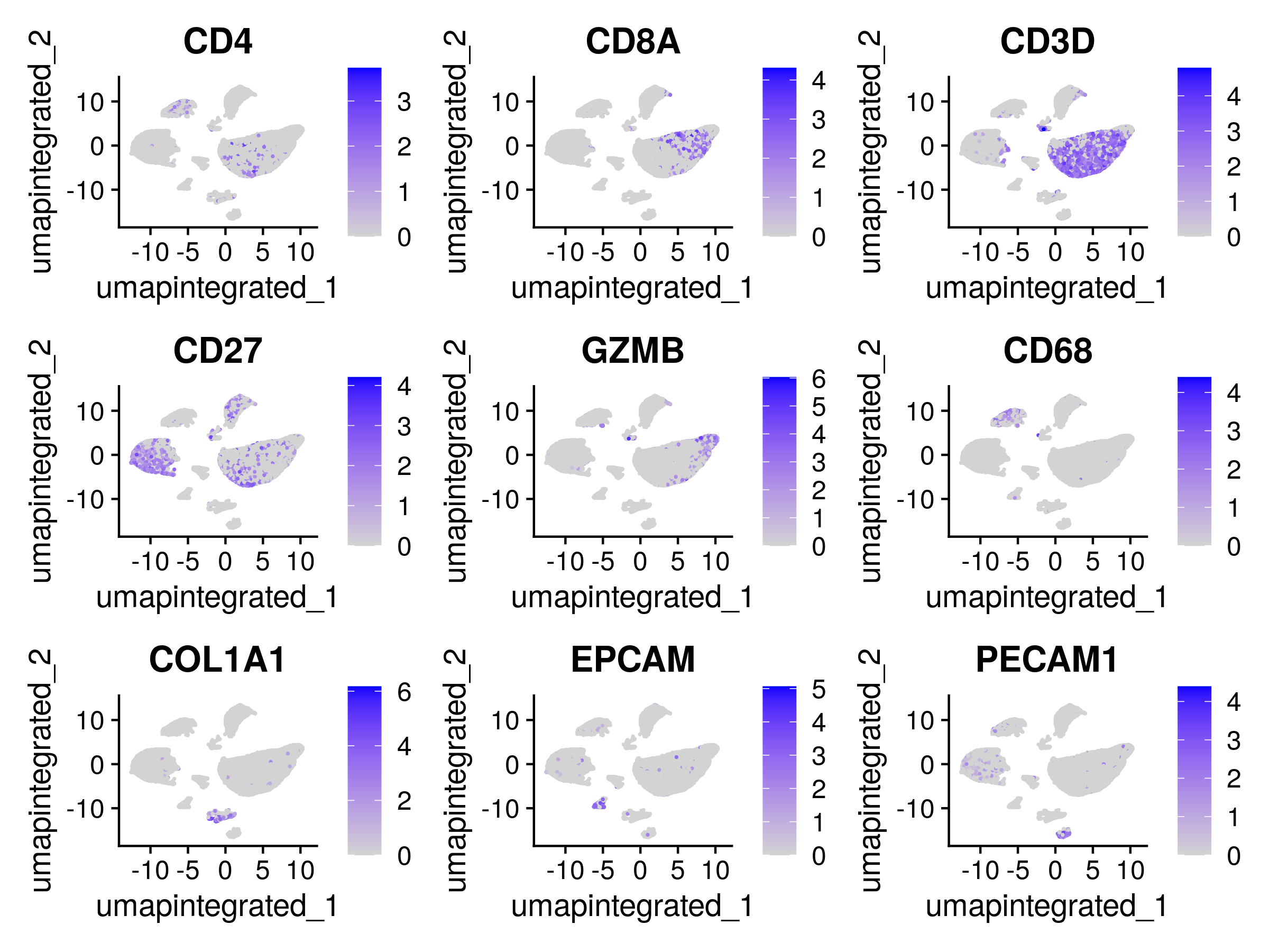
Using reference markers

p=FeaturePlot(dwIntegrated, c("CD4", "CD8A","CD3D", #Limfos
                        "CD27", #Plasma cells
                        "GZMB", #NK
                        "CD68",  #Macrophages
                        "COL1A1", #Fibros
                        "EPCAM", #Epithelial
                        "PECAM1" #Endothelial
                        ),
            reduction = "umap.integrated")
ggsave(file.path(data_dir,"figure-gfm/FeaturePlot.png"),plot = p,width = 8,height = 6)

web_summary

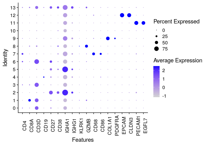
Dotplots are very useful to evaluate markers genes across clusters. They depict both the average expression (color) and the percentage of cells expressing the gene (size):

# Check Marker Genes with annother visualization
DotPlot(dwIntegrated, c("CD4", "CD8A", #Tecells
                        "CD3D", "CD19", #Bcells
                        "CD27", "CD38","IGHA1","IGHG1", #Plasma cells
                        "KLRK1", "GZMB", #NK
                        "CD68", "CD86", #Macrophages
                        "COL1A1", "PDGFRA",#Fibros
                        "EPCAM", "CLDN3", #Epithelial
                        "PECAM1", "EGFL7" #Endothelial
                        ),
        group.by = "seurat_clusters")+
  theme(axis.text.x=element_text(angle = 90))

Using a reference

When a reference dataset is available, it can be used to analyze query datasets through tasks like cell type label transfer and projecting query cells onto reference UMAPs. Notably, this does not require correction of the underlying raw query data and can therefore be an efficient strategy.

Seurat implements the projection of reference data (or meta data) onto a query object with the FindTransferAnchors and TransferData functions. After finding anchors, we use the TransferData() function to classify the query cells based on reference data (a vector of reference cell type labels), without modifying the query expression data (in contrast to integration methods). TransferData() returns a matrix with predicted IDs and prediction scores, which we can add to the query metadata with AddMetaData() function.

The package scRNAseq in Bioconductor is an alternative workflow to annotate our dataset with a reference. SingleR identifies marker genes from the reference and uses them to compute assignment scores (based on the Spearman correlation across markers) for each cell in the test dataset against each label in the reference. Due to incompatibilities between dependencies with other packages, we do not use it in this tutorial, but we acknowledge it as a good alternative.

For this tutorial, we have chosen the ifnb dataset as reference. It is available in SeuratData package an contains annotated PBMC cells. We will need to process it before:

library(SeuratData)
#InstallData("ifnb")
data("ifnb")
ifnb <- UpdateSeuratObject(ifnb)
ifnb <- subset(x = ifnb, subset = stim == "CTRL")
ifnb <- NormalizeData(ifnb)
ifnb <- FindVariableFeatures(ifnb)
ifnb <- ScaleData(ifnb)
ifnb <- RunPCA(ifnb)
ifnb <- RunUMAP(ifnb, reduction = "pca", dims = 1:15, reduction.name = "umap.pca")
DimPlot(ifnb,group.by = "seurat_annotations")

ifnb.anchors <- FindTransferAnchors(reference = ifnb, query = dwIntegrated, dims = 1:15,reference.reduction = "pca")
predictions <- TransferData(anchorset = ifnb.anchors, refdata = ifnb$seurat_annotations, dims = 1:15)
dwIntegrated <- AddMetaData(dwIntegrated, metadata = predictions)

saveRDS(dwIntegrated, file.path(data_dir, "integrated_data.Rds"))

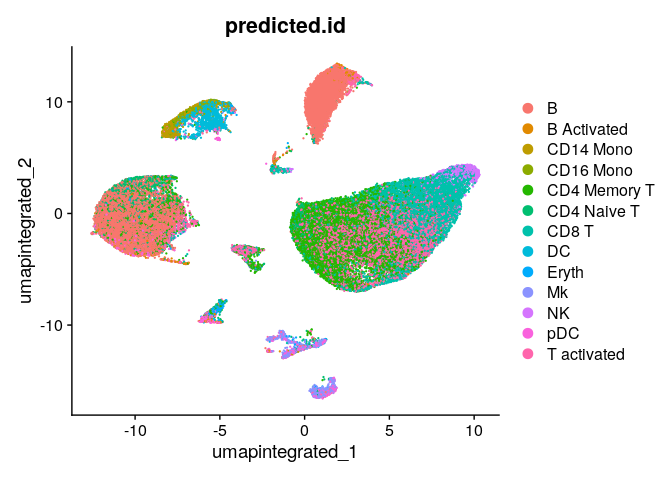
We can visualize the predicted annotations with the UMAP:

DimPlot(dwIntegrated,group.by = "predicted.id", reduction = "umap.integrated")

With this information, we are ready to annotate clusters:

new_clusters = c("T cells CD4", #0
                 "T cells CD8", #1
                 "Plasma cells", #2
                 "T cells", #3
                 "B cells", #4
                 "Plasma cells", #5
                 "T cells", #6
                 "Monocytes", #7
                 "NKs", #8
                 "Fibroblasts", #9
                 "Unknown 1", # 10
                 "Endothelial", #11
                 "Epithelial", #12
                 "Unknown 2" )#13


names(new_clusters) <- levels(dwIntegrated)
new_clusters <- factor(new_clusters,levels=c("B cells","Plasma cells",  
                                             "Endothelial", "Epithelial", "Fibroblasts",
                                             "Monocytes", 
                                             "NKs", "T cells", "T cells CD4", "T cells CD8",
                                             "Unknown 1", "Unknown 2"))


dwAnnotated = RenameIdents(dwIntegrated, new_clusters)
dwAnnotated$custom_clusters = Idents(dwAnnotated)

# Save annotated object
saveRDS(dwAnnotated, file.path(data_dir, "integrated_data_annotated.Rds"))
rm(dwIntegrated)

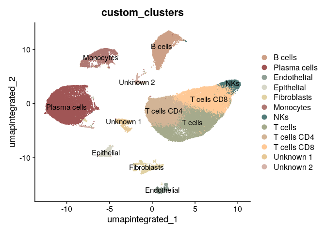
We plot the final annotated UMAP:

colors <- c("#CDA087", "#A05555", "#91A096", "#D7D7C8", "#E1D2A5", "#AF7873", 
"#527C79", "#A5AA8C", "#D2B496", "#FFC996", "#E7C897", "#D5B4AA")

DimPlot(dwAnnotated,group.by = "custom_clusters", reduction = "umap.integrated",label = T,cols = colors)

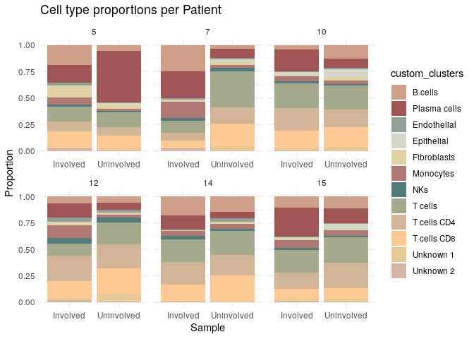
The first analysis we can perform is evaluate the cell type proportions across samples, and conditions:

library(dplyr)

prop_data <- dwAnnotated@meta.data %>%
  group_by(Sample_ID,Patient,status, custom_clusters) %>%
  summarise(count = n()) %>%
  group_by(Sample_ID) %>%
  mutate(proportion = count / sum(count)) %>%
  ungroup()

prop_data$Patient <- as.factor(prop_data$Patient)
prop_data$Sample_ID <- as.factor(prop_data$Sample_ID)

# Plot by patient
ggplot(prop_data, aes(x = status, y = proportion, fill = custom_clusters)) +
  geom_bar(stat = "identity", position = "stack") +
  scale_fill_manual(values = colors) +
  facet_wrap(~ Patient, scales = "free_x")+
  labs(title = "Cell type proportions per Patient",
       x = "Sample", y = "Proportion") +
  theme_minimal() 

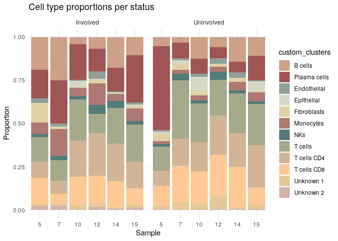
# Plot by status
ggplot(prop_data, aes(x = Patient, y = proportion, fill = custom_clusters)) +
  geom_bar(stat = "identity", position = "stack") +
  scale_fill_manual(values = colors) +
  facet_wrap(~ status, scales = "free_x")+
  labs(title = "Cell type proportions per status",
       x = "Sample", y = "Proportion") +
  theme_minimal() 

Differential expression

Differential expression analysis is the process of identifying genes that have a significant difference in expression between two or more groups. For many sequencing experiments, regardless of methodology, differential analysis lays the foundation of the results and any biological interpretation.

Different tools can be used for differential gene expression analysis, depending on the underlying statistics. One of the best known statistical tests is the Student’s t-test, which tests for how likely it is that two sets of measurements come from the same normal distribution. However, this does assume that the data is normally distributed, meaning that the data has the distinctive bell curve shape. Should this assumption be inconsistent, a non-parametric version of this test is the Wilcoxon rank-sum test, which tests how likely it is that one population is larger than the other, regardless of probability distribution size. Alternative distribution shapes can include bimodal or multimodal distributions, with multiple distinct peaks, and skewed distributions with data that favors one side or another.

For many sequencing experiments, the assumption of normality is rarely guaranteed. Some of the more popular tools for bulk RNASeq experiments, such as DESeq2, limma, and edgeR, acknowledge this, and use different statistical models to identify and interpret differences in gene expression. Single cell RNASeq is notorious for not having a normal distribution of gene expression. For technical reasons, scRNASeq has a transcript recovery rate between 60%-80%, which naturally skews the gene expression towards the non-expressed end. The Seurat tool acknowledges this, and by default uses the Wilcoxon rank-sum test to identify differentially expressed genes.

FindAllMarkers and FindMarkers

The function FindAllMarkers performs a Wilcoxon plot to determine the genes differentially expressed between each cluster and the rest of the cells (eg. cluster 5 vs all other clusters). This is useful for cluster annotation, but it takes time and we will not run it now.

Instead, FindMarkers function allows to test for differential gene expression analysis specifically between 2 groups of cells, i.e. perform pairwise comparisons, eg between cells of cluster 0 vs cluster 2, or between cells annotated as T-cells and B-cells.

We will use it to try to annotate the “Unknown” clusters, and to find differences between Plasma Cells of Involved and Uninvolved samples.

# Set annotated clusters as main Identity
Idents(dwAnnotated) <- dwAnnotated$custom_clusters
Unknown1 <- FindMarkers(dwAnnotated, ident.1 = "Unknown 1",  only.pos = T, verbose = T, min.pct = 0.1, logfc.threshold = 0.25)


# Subset Plasma cells
PC <- subset(dwAnnotated, subset = custom_clusters == "Plasma cells")
# Set status as main Identity
Idents(PC) <- PC$status
PC_de <- FindMarkers(PC, ident.1 = "Involved", ident.2 = "Uninvolved", only.pos = F, verbose = T, min.pct = 0.1, logfc.threshold = 0.1)

# Check how many DEG we get
sum(PC_de$p_val_adj <  0.05)

saveRDS(PC_de, file.path(data_dir, "PC_de.Rds"))

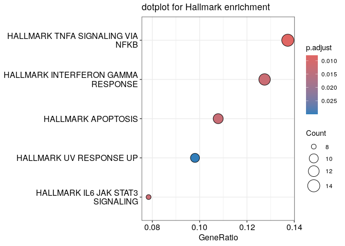
The clusterProfiler package provides functions for over-representation analysis of gmt files. We will download Hallmark gene sets from the MSigDB, This collection summarizes and represents specific well-defined biological states or processes and display coherent expression. clusterProfiler also implements Gene Ontology gene sets (among other functions, including functions for actual GSEA) or KEGG gene sets.

library(clusterProfiler)
hall_url <- "https://data.broadinstitute.org/gsea-msigdb/msigdb/release/2024.1.Hs/h.all.v2024.1.Hs.symbols.gmt"
# Download the file to a temporary location
temp_file <- tempfile(fileext = ".gmt")
download.file(hall_url, temp_file, mode = "wb")
hall <- read.gmt(temp_file)

# Subset up-regulated genes
PC_de_up  <- subset(PC_de,
                    PC_de$avg_log2FC > 1 & PC_de$p_val_adj <  0.05)
PC_de_up_genes <- rownames(PC_de_up)

# Perform enrichment 
PC_de_up_genes_HALL <- clusterProfiler::enricher(PC_de_up_genes,TERM2GENE = hall)
# Visualize significant genesets
dotplot(PC_de_up_genes_HALL) + ggtitle("dotplot for Hallmark enrichment")

Pseudobulk Differential Expression

One particular critique of differential expression in single cell RNASeq analysis is p-value “inflation,” where the p-values get so small that there are far too many genes exist with p-values below 0.05, even after adjustment. This is caused by the nature of scRNASeq, where each individual cell essentially consists of a single replicate; as the replicate count increases, the p-values tend to shrink. One method to counter the p-value inflation is to run a pseudobulk analysis. In this process, the total gene counts for each population of interest is aggregated across cells, and then these total counts can be treated in the same manner as a bulk RNASeq experiment.

pseudobulk <- AggregateExpression(object = dwAnnotated, group.by = c('custom_clusters', 'status',"Patient"),return.seurat=T)

# Subset Plasma cells
PC <- subset(pseudobulk, subset = custom_clusters == "Plasma cells")

library(edge)
y <- DGEList(PC@assays$RNA$counts, samples=PC@meta.data)
# Set status as main Identity
Idents(PC) <- PC$status

PC_df <- FindMarkers(PC, ident.1 = "Involved", ident.2 = "Uninvolved", only.pos = F, verbose = T, min.pct = 0.1, logfc.threshold = 0.1,test.use = "DESeq2")


# Check how many DEG we get
sum(na.omit(PC_df$p_val_adj <  0.05))